Appraiser formfilling at its best with rock solid stability, a highly intuitive interface, and blazing speeds
Developing reports is the cornerstone of your business. With more and more client demands, you need software that won’t slow you down. More appraisers choose TOTAL because it’s intuitive, stable, built for today’s technology (it runs beautifully on Windows 10), and includes the features that save you the most time on every report.
Superior Side-by-Side Comps
Our Comps Side-by-Side PowerView shows all your comps, rentals, and listings on one scrolling screen. Adding, editing, and removing is effortless, and you can drag and drop the comps themselves to change their order on your screen at any time. Discarded comps are even stored in your report’s Spectrum Workfile in case you get asked why you didn’t use a particular property later or if a request comes in for even more comps.
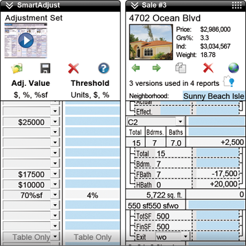
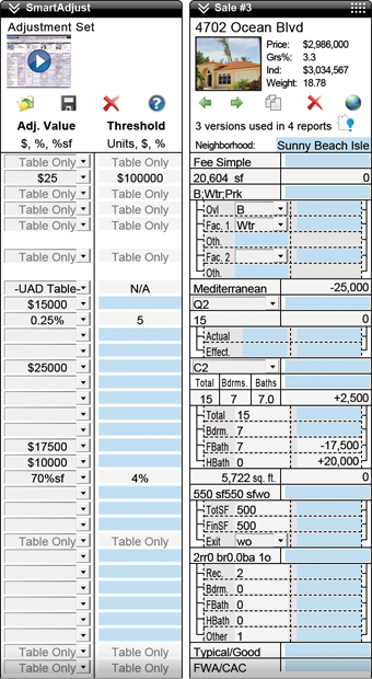
Auto adjustments on steroids
SmartAdjust is the only adjuster that handles both numeric and non-numeric adjustments, and does so for both UAD and non-UAD reports in one consistent interface. You’ll save time on every field in the grid — especially the compound UAD fields, like basements and bathrooms, which we automatically break out into separate line items for you to apply individual adjustment factors.
So, for bathroom count you’ll see one SmartAdjust sub-line for the full baths, plus one for the half baths, and you'll adjust your factors separately for each. Factors are applied to all comps at once.
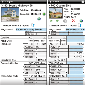
Save time in the comps grid
Adjusting comps has become more of a hassle since UAD, forcing you to keep a separate spreadsheet just to break down adjustments for items such as partially-finished basements. Our Detailed View breaks down each field in the grid into individual line-items. For instance, enter the finished basement square footage and total square footage, along with any rooms below grade, and adjust each one accordingly. Details are saved to your workfile in case you’re questioned by auditors later.
Stuck in a contract with another appraisal software vendor?
Switch to TOTAL and we'll buy out your existing contract
With our Buyout Program, get a prorated discount on TOTAL for what you've already paid your software vendor over the past 12 months. You could even switch for free!
“You have such a great team of professionals. I am so glad I came over from ACI. I've been with a la mode for several years, and you're the best.”
Tom Gress, Appraisal Co.
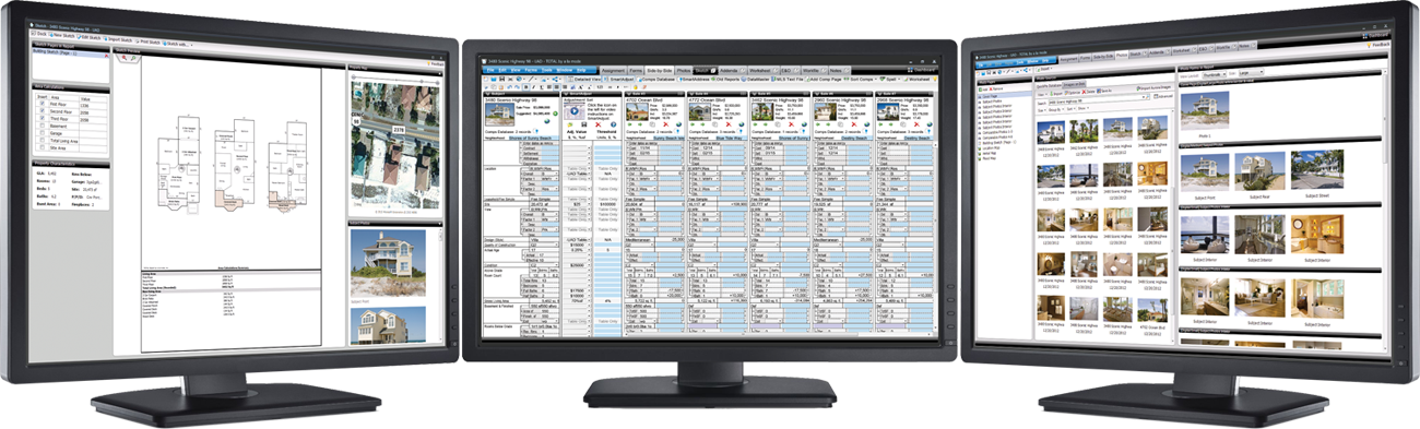
Work with multiple monitors seamlessly
With TOTAL’s modern, multi-window functionality, you can open multiple live, active windows on one appraisal — or on several different reports at a time — and work between screens effortlessly. When you make a change to your report in one TOTAL window, all the others will update in real time.
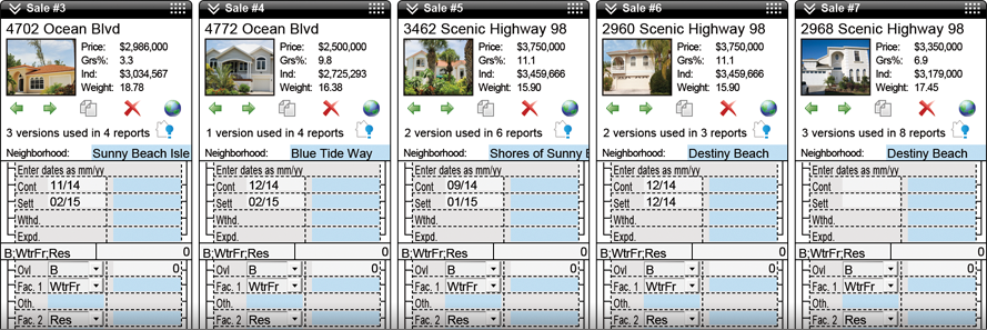
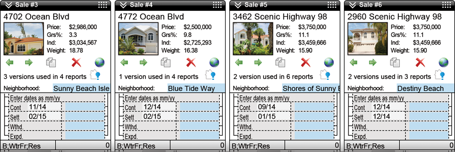
Save time and ensure consistency with SmartAddress
SmartAddress instantly alerts you to subject and comp properties you’ve used before so you can easily pull in prior data and check for inconsistencies. With one click, SmartAddress displays side-by-side all the previous versions of a property that you’ve used (not just the most recent). This makes it easy to compare and spot inconsistencies. From there, merge entire previous records or pick and choose which field data to add to your current report.
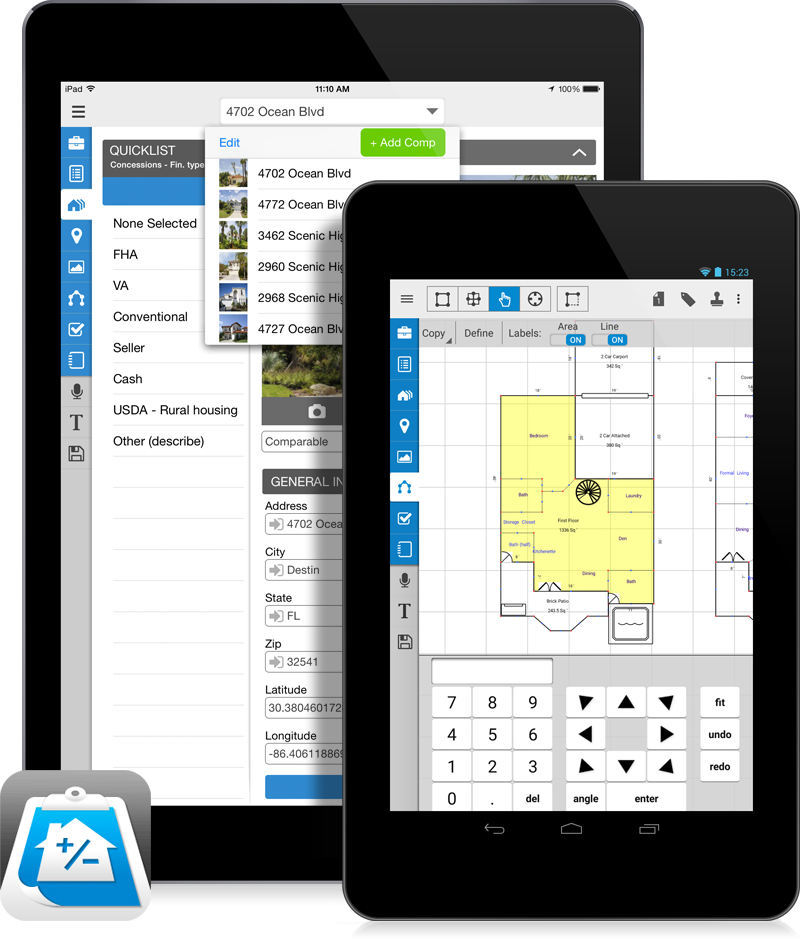
TOTAL for Mobile™ — better syncing, photo tools, and more
We’ve built our own mobile tools to work seamlessly with our desktop products. All the field data you collect (including voice notes, photos, sketches, and more) on your iPad® or Android™ device flows into your TOTAL report and your Spectrum Digital Workfile — you’ll save an incredible amount of time from field to office by not having to retype, resketch, and reformat.
Your forms are literally at your fingertips, including the complete 1004, 1004 UAD, 2055 UAD, Condo, Land, and Canadian AIC. You’ll also find the 1025 and our exclusive General Purpose Residential Form for non-lender clients. We’re also adding more popular forms and customer-requested features and improvements.
Bottom line: You’ll be completely paperless and won’t need a clipboard again.
The most advanced Comps Database
Integrate all data sources (prior reports, MLS data, public records, photos, notes, and more) into one comprehensive view of your market.
Sales, rentals, and listings automatically fill your database with properties from every report, giving you a complete history of your comps.
Searching is world-class. Simply “draw” any shape on the map to immediately find the most likely comps by
default every time.

A superior way to organize reports
You’ve probably had to access reports you did in the past on occasion in your career. Did you remember the file names of those reports you worked on months or years before? Your appraisal reports shouldn’t be saved and sorted like traditional documents. With TOTAL’s Appraisal Desktop, you can easily search, sort, and display reports by address, borrower name, client name, and dozens of other criteria. Best of all, when you select a report, you’ll see details without having to open the file — including a preview of the report, the invoice, order information, much more.
Fire up new reports in no time
If you like to just “get in and go”, you’ll love TOTAL. Simply click “File”, then “New”, and you’re off to the races in about five seconds. Enter the subject address and then choose how much (or little) information you want to enter up-front. From there, choose to dive straight into your form. Or, if you don’t want to start from scratch, use SmartMerge to pull in data from old reports or templates in a snap. No more time wasted
retyping old reports.
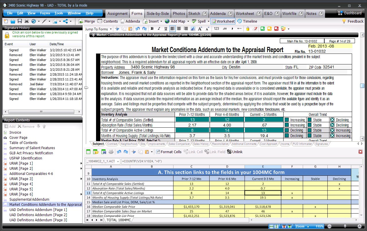
Cut calculation time with integrated Worksheets
TOTAL’s Worksheets are one of the most powerful features of any appraisal formfiller. If you’ve worked with spreadsheets, you know the value of being able to calculate data instantly. But then you have to copy and paste that data into your form.
Worksheets are built into TOTAL, so your calculations flow directly into your forms. Create your own or use our ready-made 1004MC template to completely automate your Addendum.
Spectrum Digital Workfile Architecture — the proper way to go paperless
Our Digital Workfile PowerView makes building your report simple. Simply browse and select, drag and drop, or paste files to your report from inside the Workfile PowerView. Include any file – photos, MLS comp sheet PDFs, emails, scanned documents, faxes, and more. (TOTAL also adds files automatically, such as the delivered PDF, comps that didn’t make the cut, and TOTAL for Mobile inspection data.) Everything is saved with your report and easily flows Titan Drive.
Later, if questioned by an underwriter or auditor (much more common these days, even years later), simply pull up your Digital Workfile from the cloud instead of sifting through emails or expensive paper file cabinets.
Sketch PowerView: Quickly fly through your sketch
Our Sketch PowerView was designed knowing that you might inspect properties a few days before you add your sketch in the report. You may not remember every minute detail, so we made it super simple to have the rest of your report open for easy reference.
Addenda PowerView: Robust, integrated word processor
Text overflows to your addenda in the same sequence the fields appear on the form, making it much easier for you and your clients to read. You can also quickly insert external pieces such as Word docs, images, charts, and tables into any section of your addenda.
Assignment PowerView: Manage assignments with ease
In the Assignment PowerView you have quick access to everything related to your report — add or delete invoices, see your order form with a map and driving directions, review instructions from the client and more. You'll even see FEMA and census data up front.
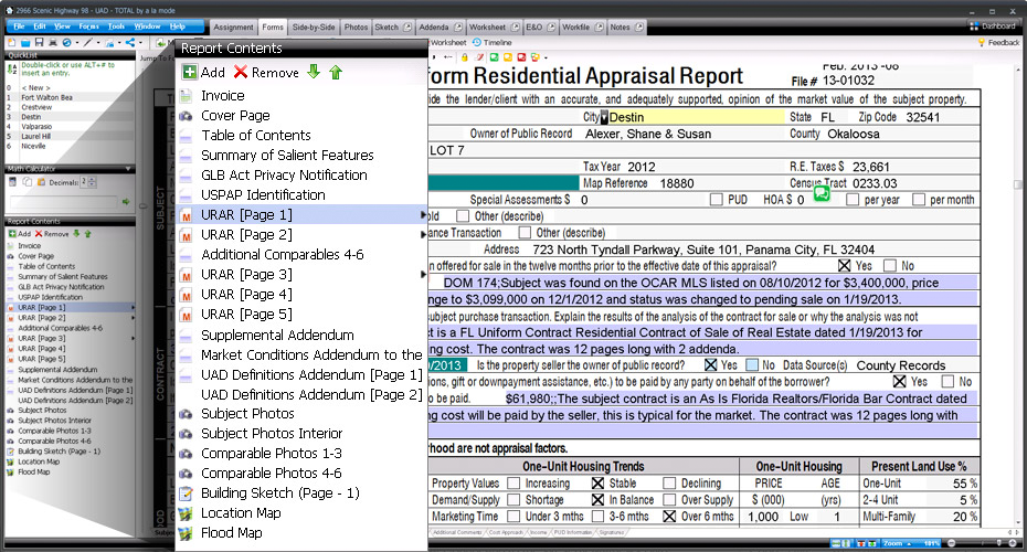
Quickly navigate and manage your forms with ease
Most people spend the majority of their time in TOTAL looking at the forms screens. That’s why we paid careful attention to improving the speed and navigation in the Forms PowerView.
TOTAL’s Report Contents panel keeps all the forms in your report visible and instantly accessible. Quickly add or remove forms, jump to a specific page, or rearrange everything without ever leaving
the Forms PowerView.
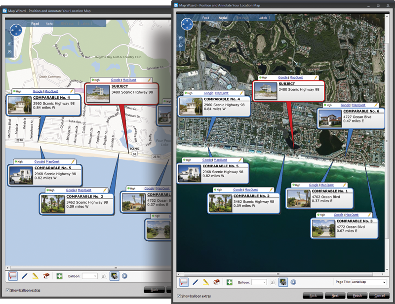
Unlimited location maps, flood, and census data
Other vendors charge appraisers on a per-map basis for location maps, or require flood map subscriptions to get any flood data. TOTAL comes with truly unlimited location maps, aerial and street maps, as well as flood data and census tracts with scrubbed addresses. Flood and census data automatically flows into your report when you enter the property address. You don’t have to look anything up.
With TOTAL’s mapping options, see all your comps on one map, get driving directions from your office, and automatically standardize USPS data from all of the properties into your report.
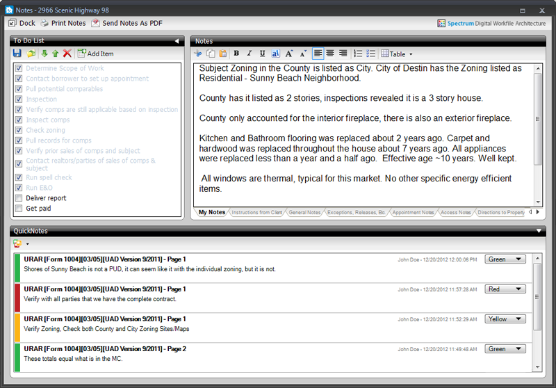
Ditch your paper notes and scattered to-do lists
You probably have a list of items you check in every report. To stay organized, use the Notes PowerView. It keeps you focused, paperless, and USPAP-compliant by storing all your notes and tasks in your report’s Digital Workfile. No other vendor has anything like it. You’ll add QuickNotes (digital sticky notes) to your form, and they show up in the Notes PowerView where they can be reviewed, edited, and printed. And your clients won’t be able to see anything from your notes either.
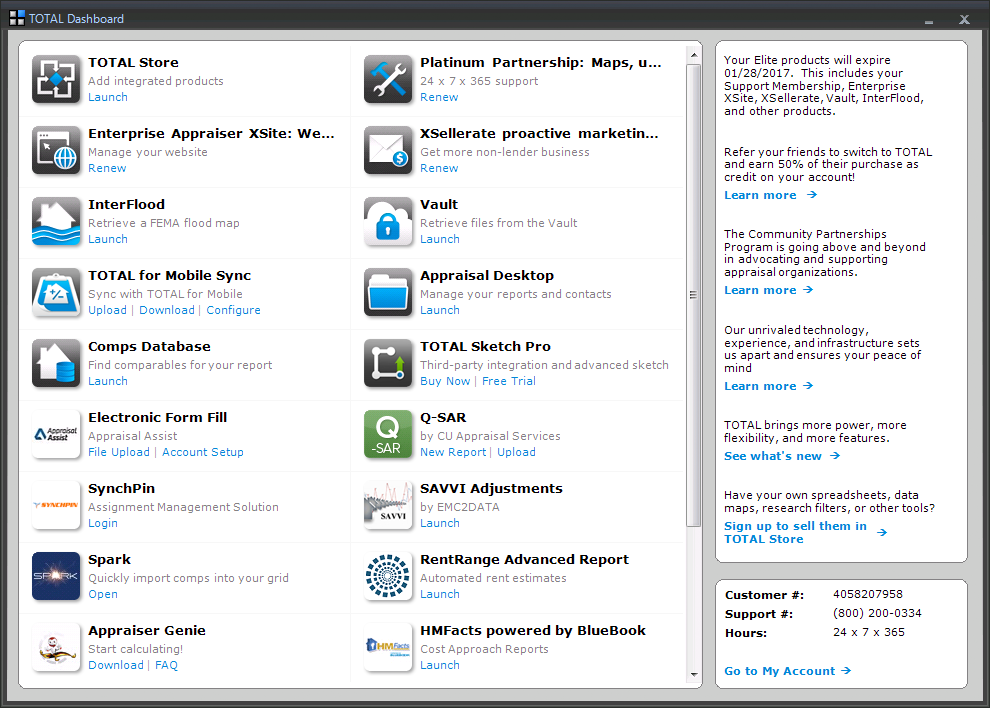
Instant access to your suite of tools with the Dashboard
You shouldn’t have to exit your formfiller to launch other apps or sites that work with it. That’s why TOTAL makes integration with third party apps easy. Simply click the Dashboard button in TOTAL’s toolbar and you’ll have instant access to your appraisal apps without all the extra clicks, browsing, or confusion on how to launch a program. You’ll even have quick access to your account details including tech support phone numbers and hours.
Our newest forms engine is faster and more precise
Everything about TOTAL was engineered to be faster. TOTAL was designed to fully maneuver today’s hardware, and it now loads reports more than four times faster than previous versions. And that’s not all. The program itself loads quicker, scrolls faster, and merges data quicker. Try it side-by- side against whatever you’re using now, on the same machine, and you’ll see the difference.
Speed alone isn’t enough of course. The engine is more precise too. It’s easier to place the cursor properly in complex multi-line fields, selecting large blocks of text is more predictable, and even scrolling and jumping between forms is fine-tuned for precision. Plus, with the new rendering technology and our new High Definition fonts, forms always display in stunning clarity.
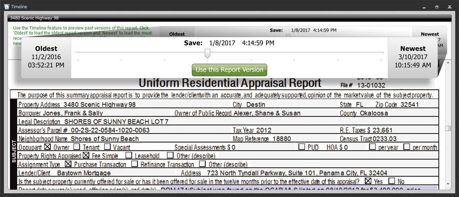
Mistakes are a thing of the past
We’ve all been there. That heart-stopping moment of losing hours of work after making a mistake — like merging data into the wrong report and saving. With TOTAL’s Timeline, never worry about those errors again.
Timeline automatically saves copies of your report in various stages as you enter data, add and swap forms, merge data, or deliver. Using Timeline, you can roll back your report to the version before you made any major change so you’ll get right back to work.
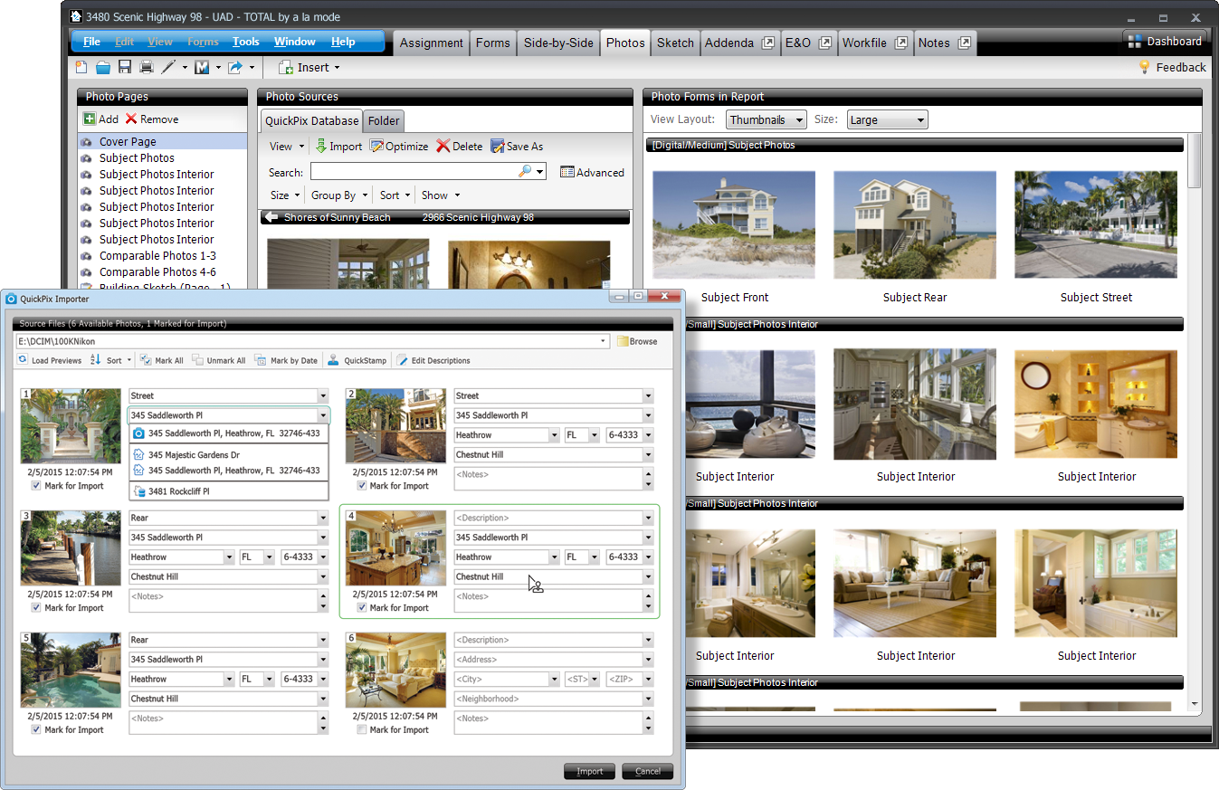
Managing photos is easier than ever with Photos PowerView and QuickPix
Put an end to manually organizing photos. The QuickPix Importer in TOTAL pulls in thumbnails from your camera or computer for you to review and quickly pick which ones to use. Then, you just have to add a description, address, neighborhood, and notes before importing them into your report. Or, let the QuickPix Importer auto-complete information using data from your open reports. And QuickStamp lets you copy all the address data from one photo and “stamp” it onto other photos with a single click.
When you add a photo to a report, all available property information is automatically added into the QuickPix Database for easy searching later. From there, you can drop the image straight into your form without worrying about entering details. In your database, photos are grouped by neighborhood, address, or date, so adding them into reports a breeze.
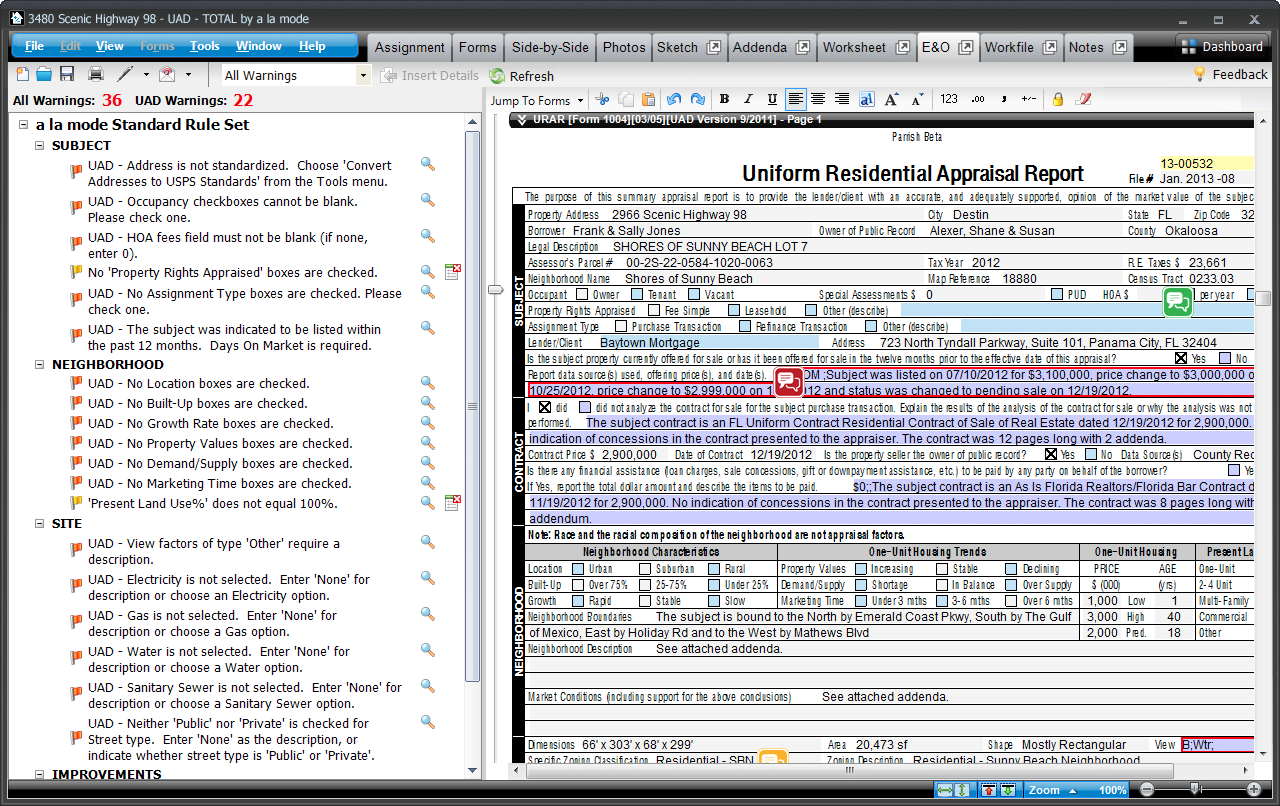
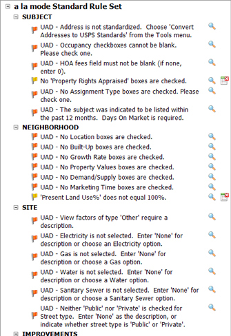
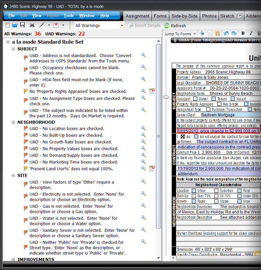
Customizable, intelligent checks and warnings using TOTAL’s E&O PowerView
Dramatically reduce annoying revision requests and present a more polished final report with TOTAL’s robust E&O PowerView. Instead of your client catching them, you’ll catch any accidental errors before your report leaves your desktop.
Rules are customizable for non-UAD warnings too. For example: When your comp age differs by more than 30%, but most of your appraisals are new construction, you can exclude that rule from the warning list. It’s extremely flexible.
Run the E&O check and click on a warning to jump to the problematic field and correct it. When you’re finished, add results as pages to your report.
“It’s been three weeks now since I switched from ACI to TOTAL. It’s really been an easy transition. I’m already completing assignments faster, and it’s only been three weeks. I am loving TOTAL! I only wish I had made the choice to switch a long time ago. a la mode’s tech support is awesome!”
The transition is easier than you think
We’ve made TOTAL incredibly easy to dive into. Open files from your current formfilling software using our simple Competitor Conversion Wizard or import UAD XML files. The converter helps you copy data into TOTAL so you don’t have to worry about retyping or starting from scratch.
TOTAL is incredibly intuitive, but if you do have questions along the way our Product Coaches will help you get acclimated in one-on-one calls. You’ll also find helpful webinars, tutorial videos, and more to teach you all the tips and tricks of saving the most time with TOTAL.